#03 · 2026
Forecasting Daily Sales Across 150 Shop-Product Combinations
AnalysisToptal screening project · LightGBM · Tweedie objective · Retail time series
46.5%
lower MAE vs. seasonal naive
150
shop–product series
61 days
forecast horizon
my_role: Individual Contributor (IC) - data exploration, feature engineering, LightGBM Tweedie model, validation and presentation.
A LightGBM Tweedie model, built and validated on four years of retail sales data. The task: build a model that predicts sales for each of the 150 shop–product pairs over a forecast window running December 2021 through January 2022 - and show the reasoning, not just the number.
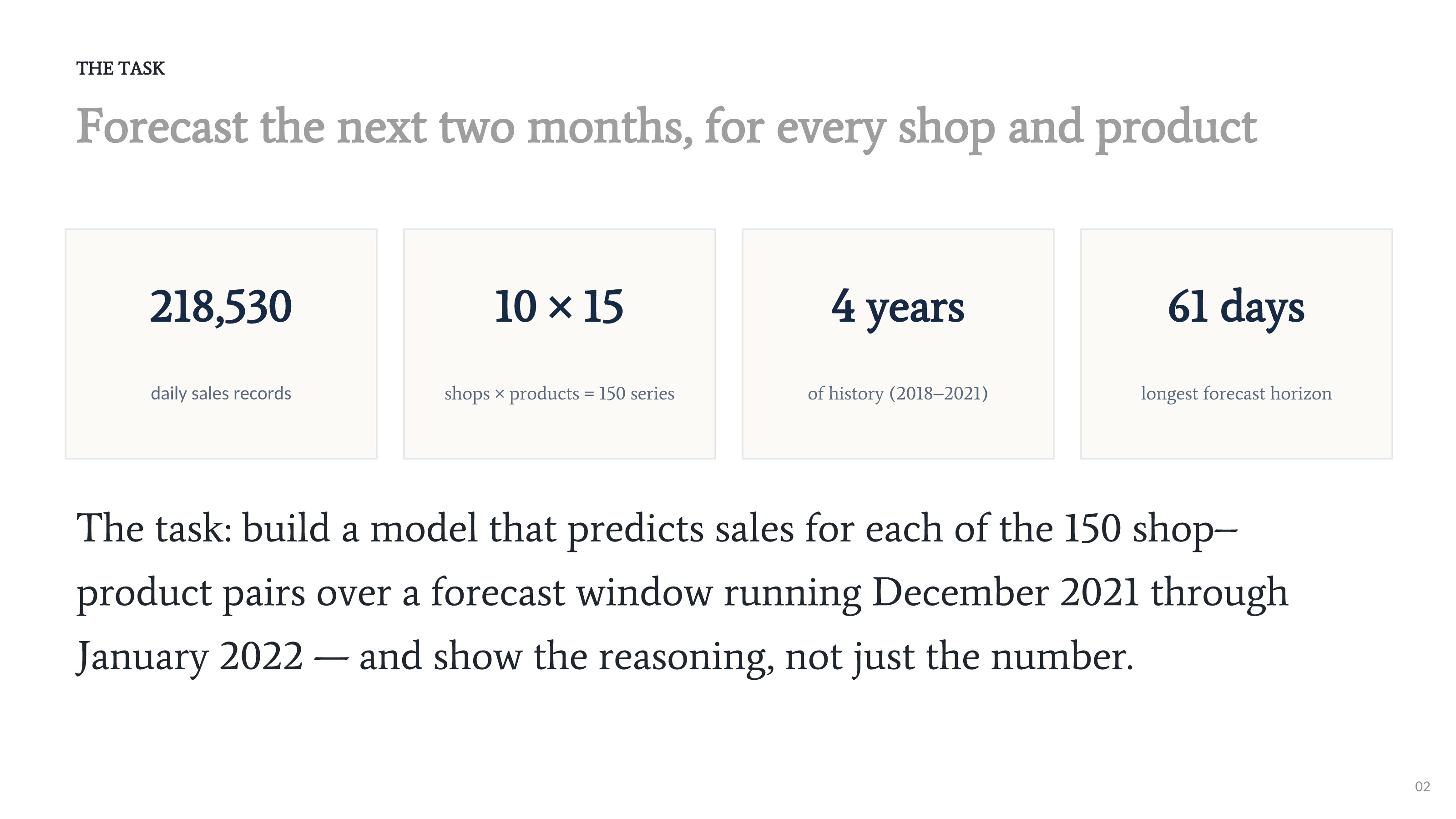
## The task - forecast the next two months
- ›218,530 daily sales records
- ›10 shops × 15 products = 150 shop–product series
- ›Four years of history (2018–2021)
- ›61 days: longest forecast horizon; target window December 2021–January 2022
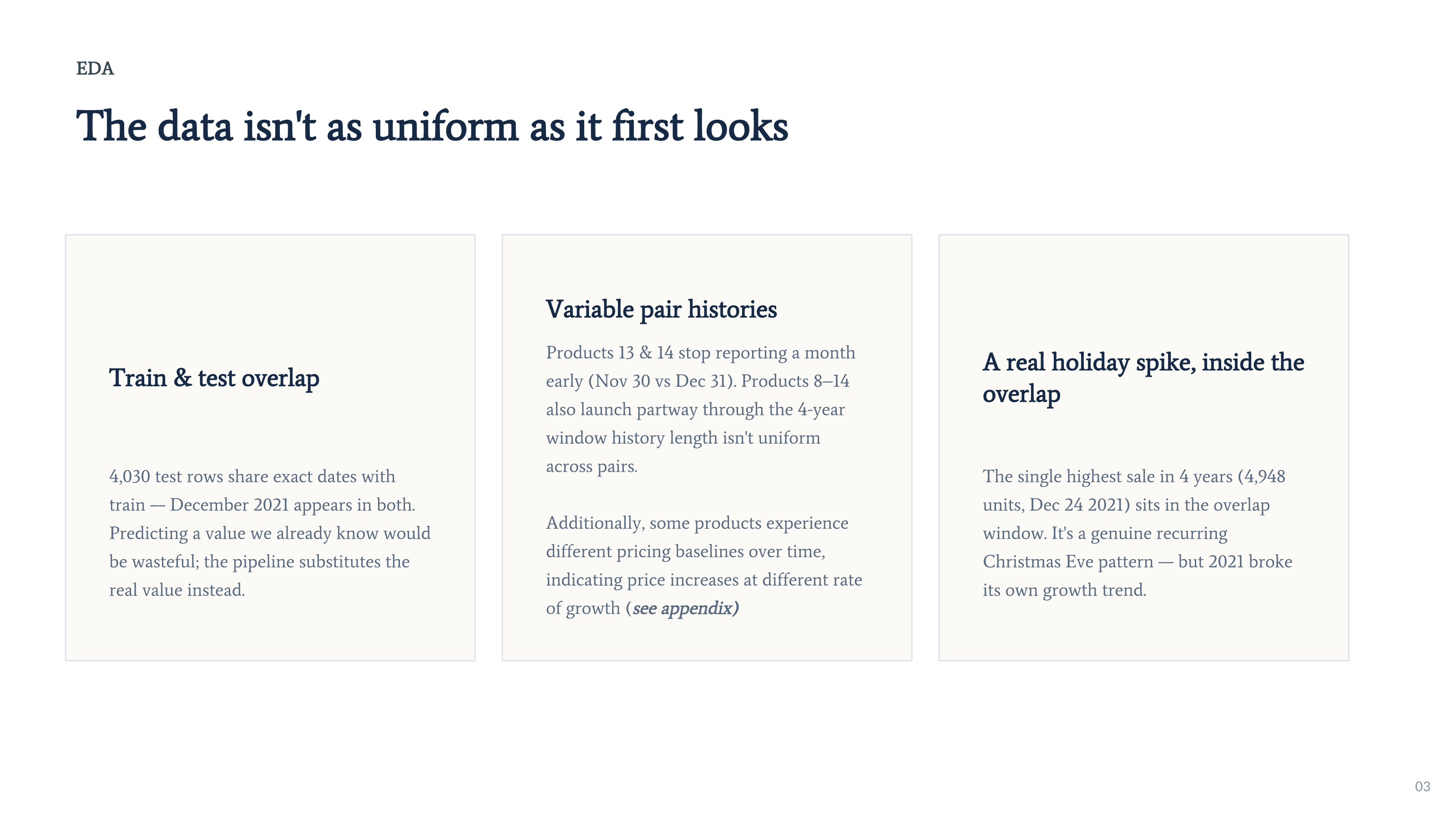
## The data isn’t as uniform as it first looks
- ›Train and test overlap: 4,030 test rows share exact dates with train - December 2021 appears in both. Predicting a value we already know would be wasteful; the pipeline substitutes the real value instead.
- ›Variable pair histories: Products 13 and 14 stop reporting a month early (November 30 vs. December 31). Products 8–14 also launch partway through the four-year window; history length isn’t uniform across pairs.
- ›Some products experience different pricing baselines over time, indicating price increases at different rates of growth.
- ›A real holiday spike, inside the overlap: the single highest sale in four years (4,948 units, December 24, 2021) sits in the overlap window. It’s a genuine recurring Christmas Eve pattern - but 2021 broke its own growth trend.
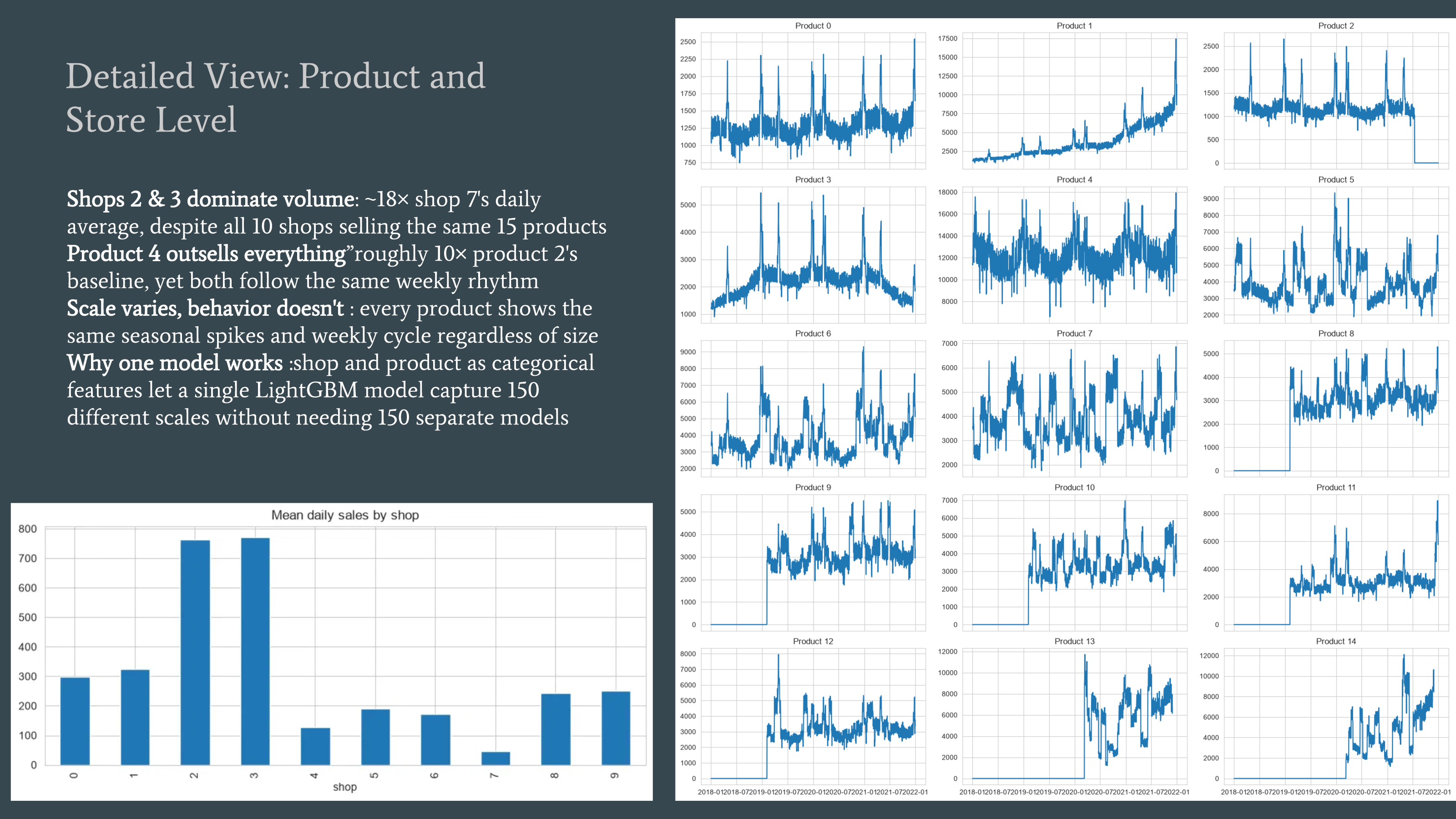
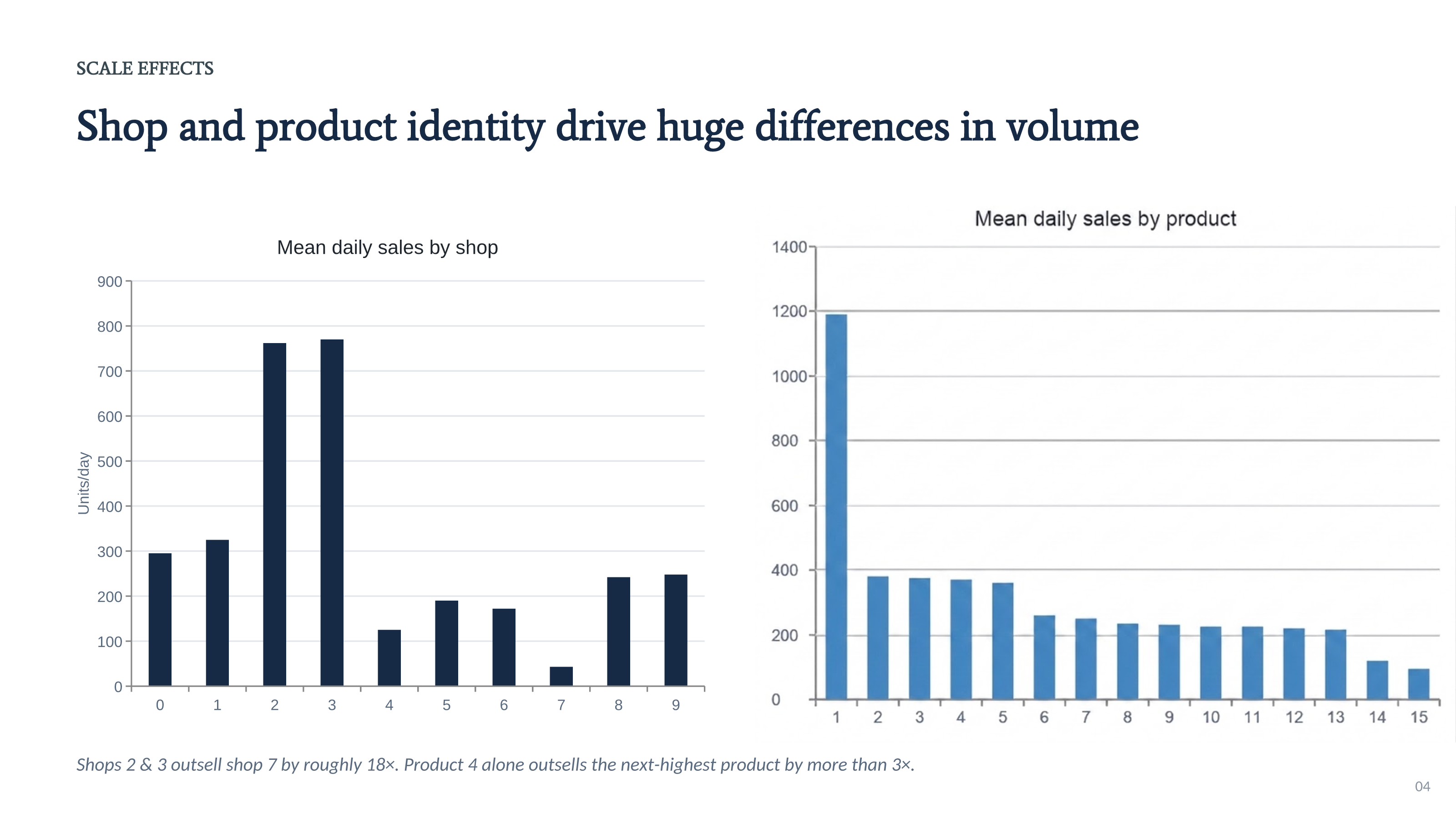
## Shop and product identity drive huge differences in volume
Shops 2 and 3 outsell shop 7 by roughly 18×. Product 4 alone outsells the next-highest product by more than 3×. The original product and shop charts are preserved with the slides.
## Zero-inflated sales, with a clear weekend lift
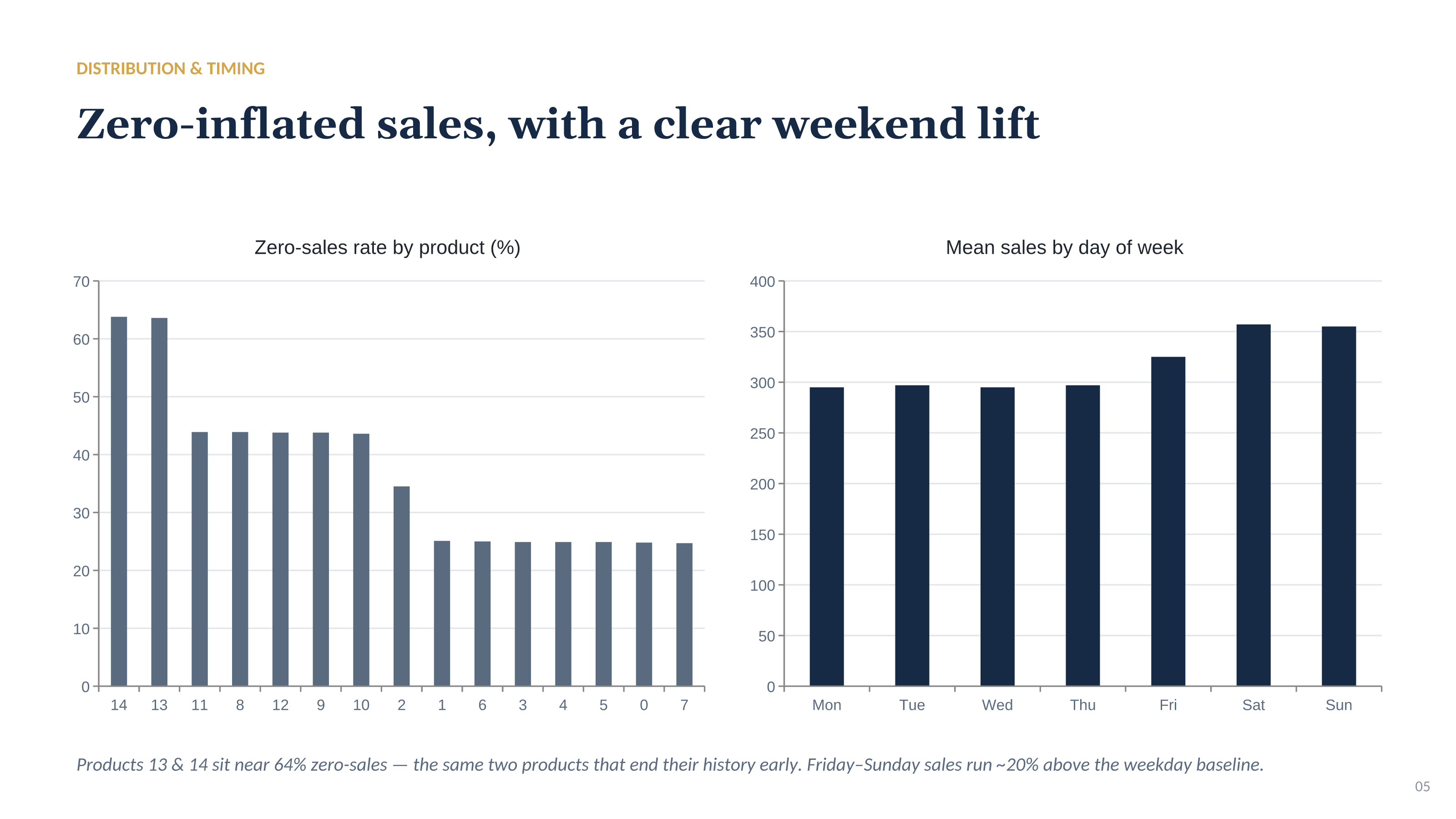
Products 13 and 14 sit near 64% zero-sales - the same two products that end their history early. Friday–Sunday sales run approximately 20% above the weekday baseline.
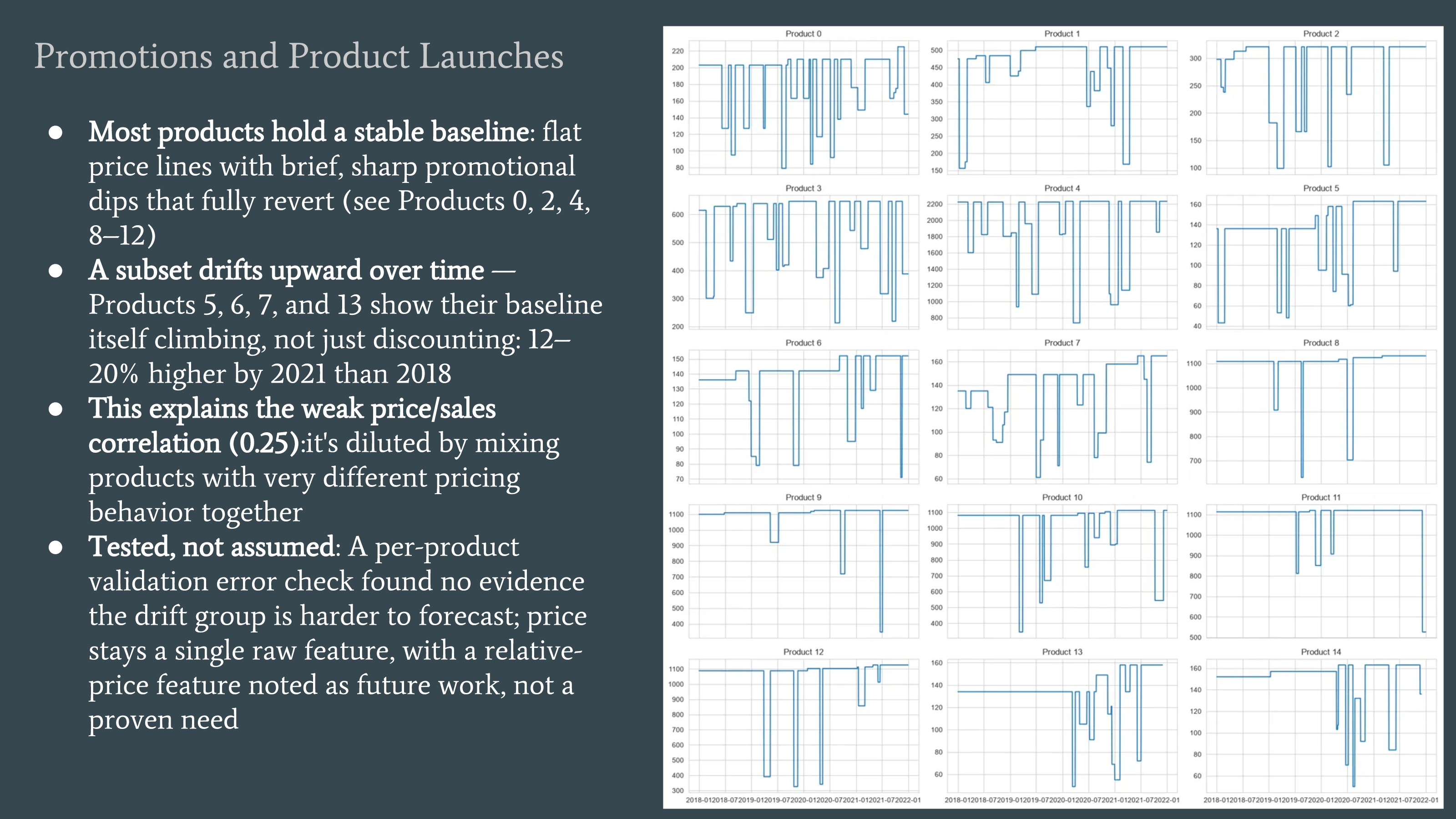
## Price isn’t static
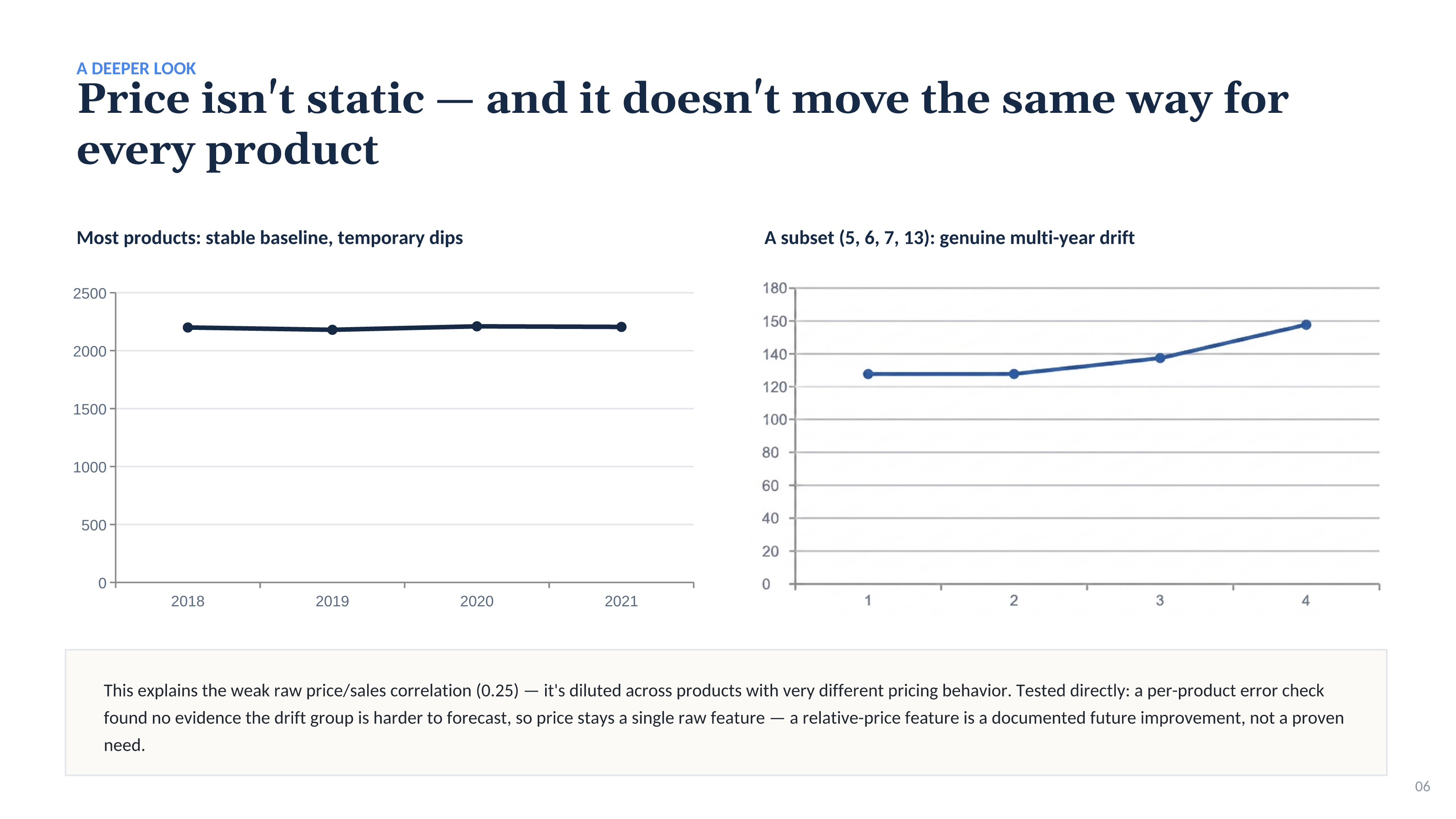
Most products have a stable baseline with temporary dips. A subset (5, 6, 7, 13) has genuine multi-year drift. This explains the weak raw price/sales correlation (0.25) - it’s diluted across products with very different pricing behavior. Tested directly: a per-product error check found no evidence the drift group is harder to forecast, so price stays a single raw feature - a relative-price feature is a documented future improvement, not a proven need.
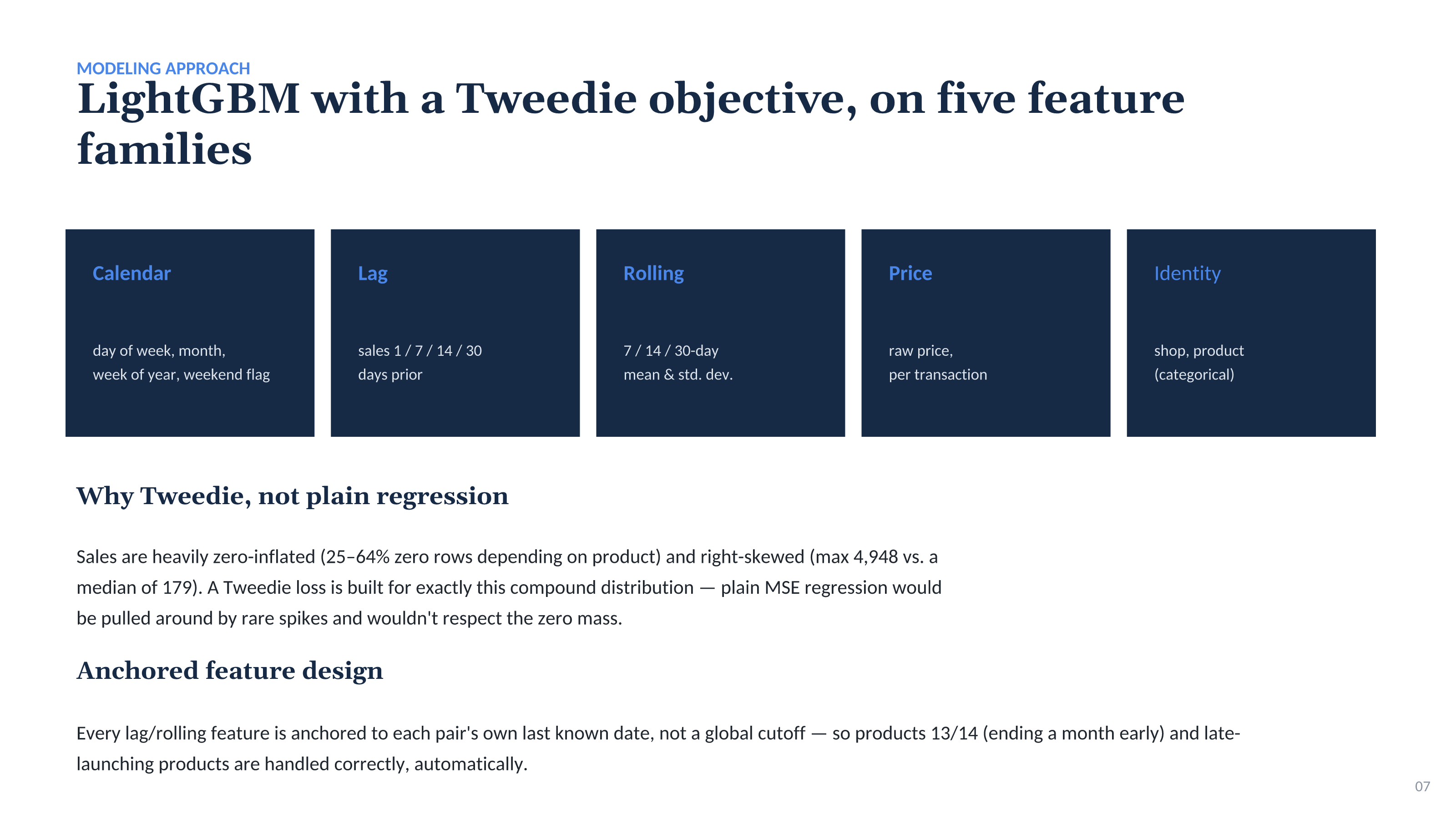
## LightGBM with a Tweedie objective - five feature families
- ›Calendar: day of week, month, week of year, weekend flag
- ›Lag: sales 1, 7, 14 and 30 days prior
- ›Rolling: 7-, 14- and 30-day mean and standard deviation
- ›Price: raw price, per transaction
- ›Identity: shop and product (categorical)
## Why Tweedie, not plain regression
Sales are heavily zero-inflated (25–64% zero rows depending on product) and right-skewed (maximum 4,948 vs. a median of 179). A Tweedie loss is built for exactly this compound distribution - plain MSE regression would be pulled around by rare spikes and wouldn’t respect the zero mass.
## Anchored feature design
Every lag/rolling feature is anchored to each pair’s own last known date, not a global cutoff - so products 13/14 (ending a month early) and late-launching products are handled correctly, automatically.
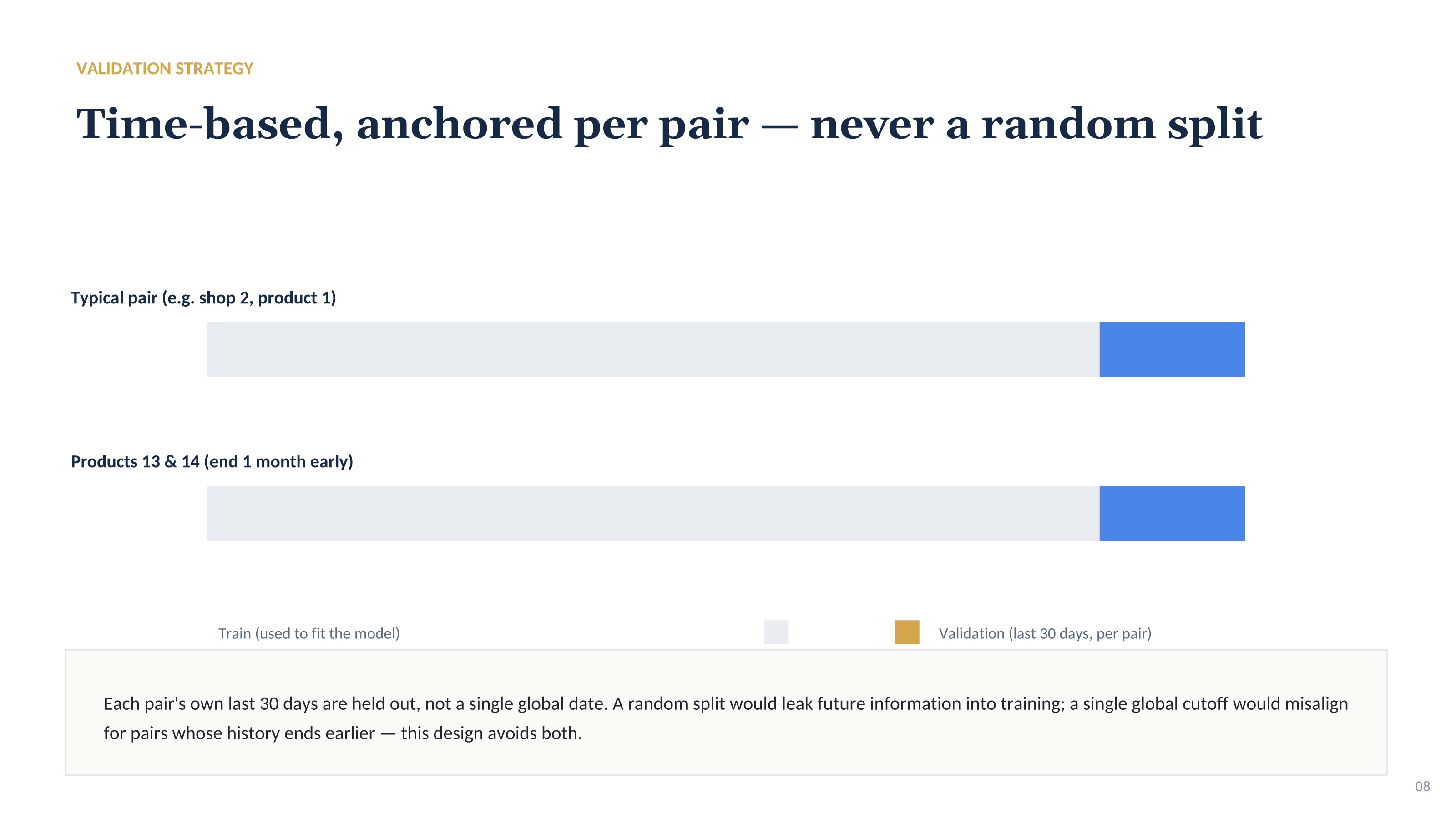
## Validation - time-based, anchored per pair
Each pair’s own last 30 days are held out, not a single global date. A random split would leak future information into training; a single global cutoff would misalign for pairs whose history ends earlier - this design avoids both.
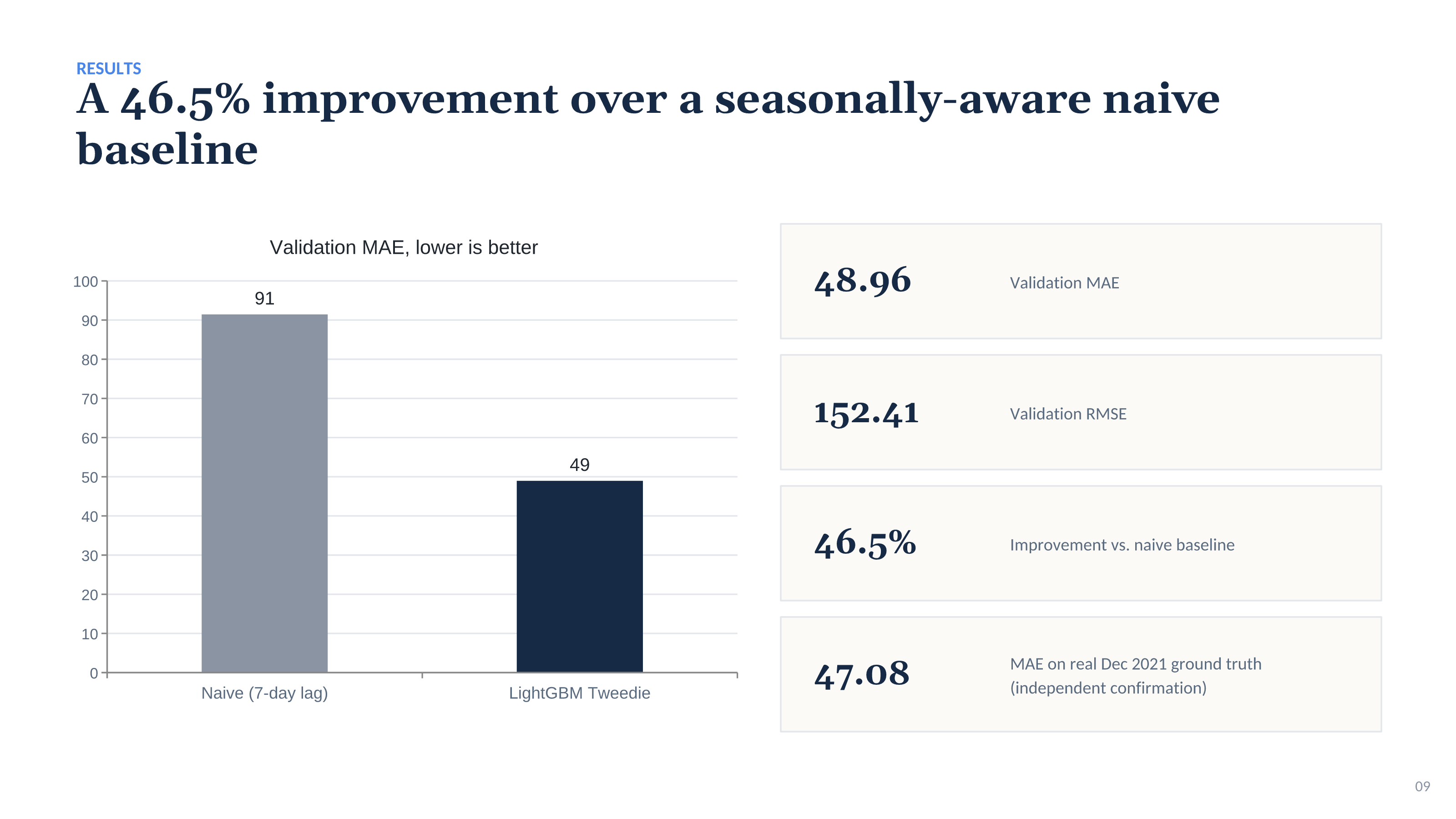
## Results - a 46.5% improvement over a seasonal naive baseline
- ›Validation MAE: 48.96
- ›Validation RMSE: 152.41
- ›Naive baseline (7-day lag) validation MAE: 91.45
- ›Improvement versus naive baseline: 46.5%
- ›MAE on real December 2021 ground truth: 47.08 (independent confirmation)
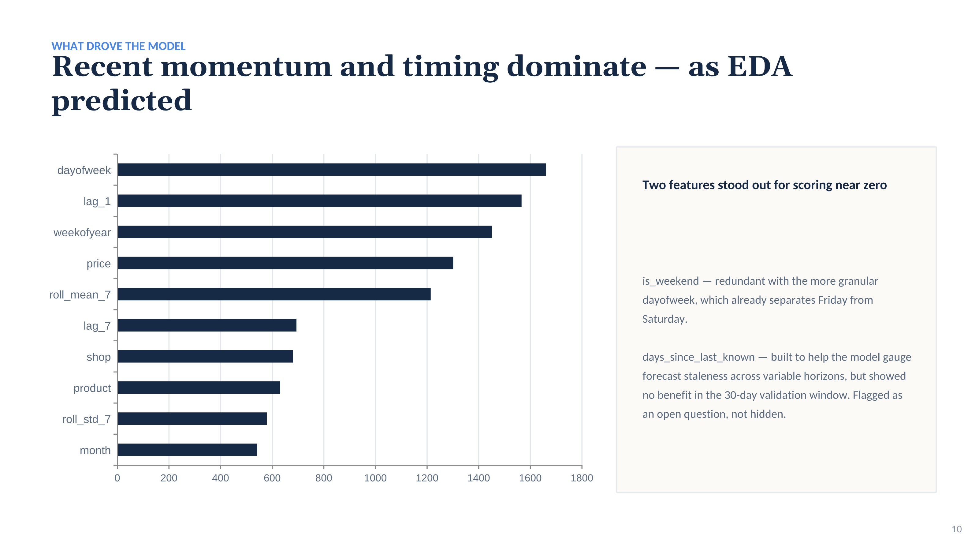
## What drove the model
Recent momentum and timing dominate - as exploratory analysis predicted.
- ›Feature importance: dayofweek 1,660; lag_1 1,566; weekofyear 1,451; price 1,301; roll_mean_7 1,214; lag_7 694; shop 681; product 630; roll_std_7 579; month 542.
- ›is_weekend scored near zero: redundant with the more granular dayofweek, which already separates Friday from Saturday.
- ›days_since_last_known scored near zero: built to help the model gauge forecast staleness across variable horizons, but showed no benefit in the 30-day validation window. Flagged as an open question, not hidden.
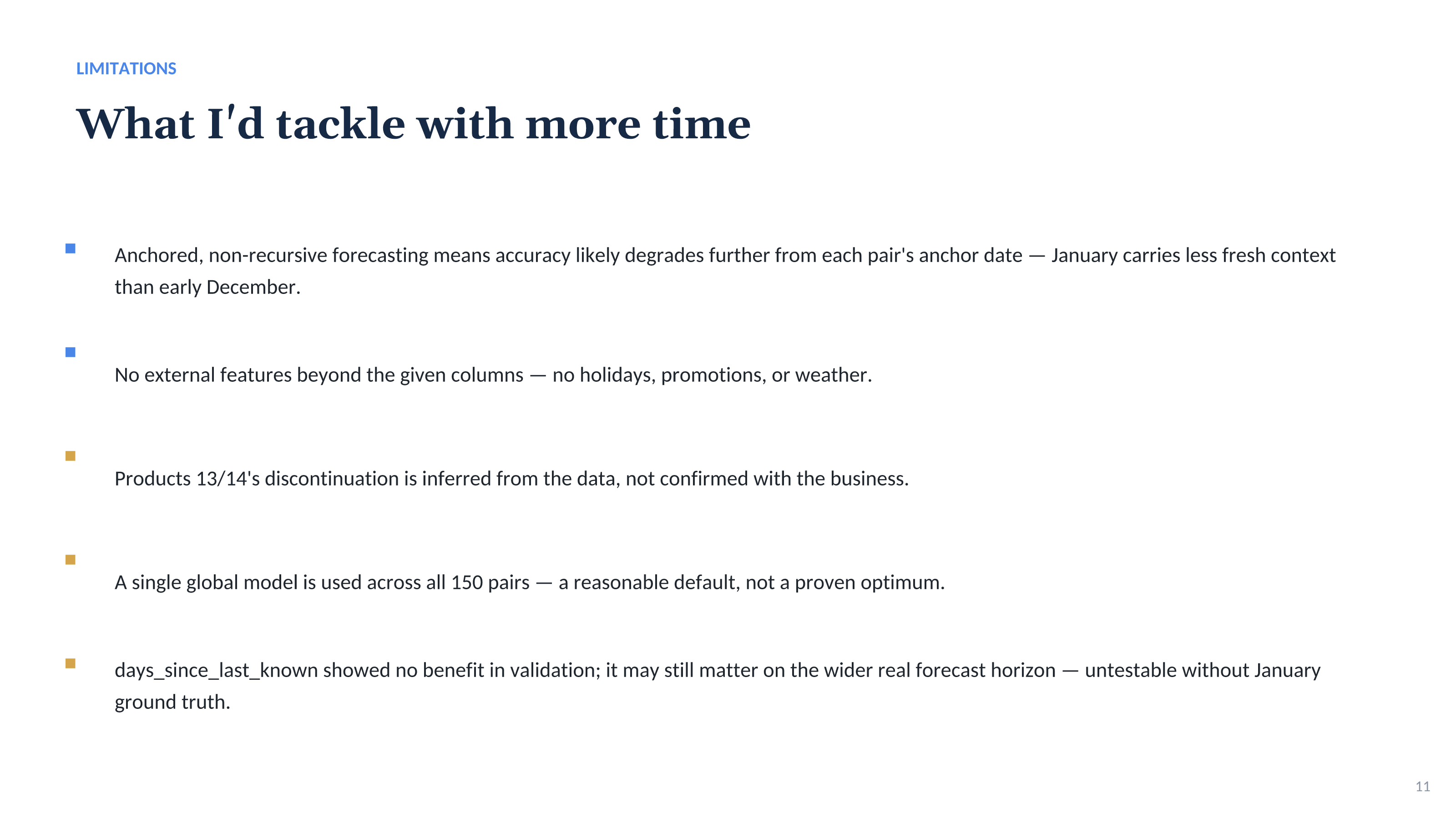
## Limitations - what I’d tackle with more time
- ›Anchored, non-recursive forecasting means accuracy likely degrades further from each pair’s anchor date - January carries less fresh context than early December.
- ›No external features beyond the given columns - no holidays, promotions or weather.
- ›Products 13/14’s discontinuation is inferred from the data, not confirmed with the business.
- ›A single global model is used across all 150 pairs - a reasonable default, not a proven optimum.
- ›days_since_last_known showed no benefit in validation; it may still matter on the wider real forecast horizon - untestable without January ground truth.
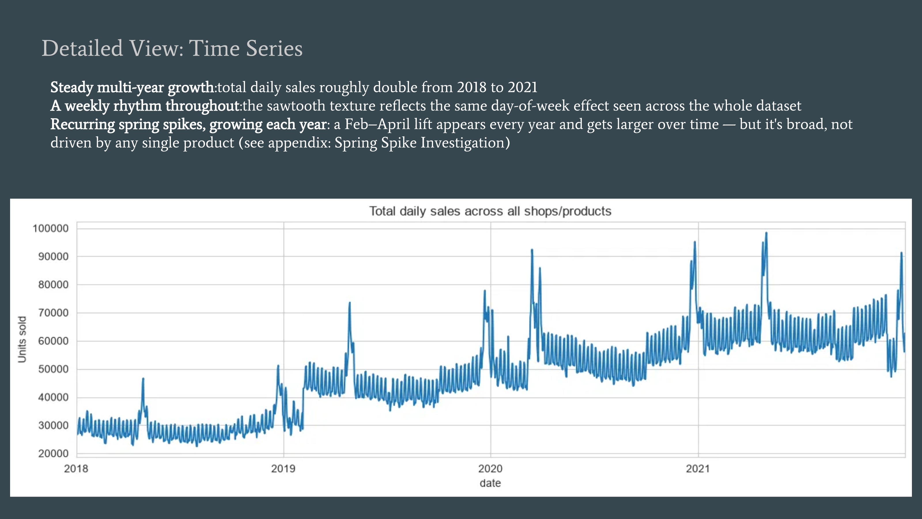
## Detailed view - time series
- ›Steady multi-year growth: total daily sales roughly double from 2018 to 2021.
- ›A weekly rhythm throughout: the sawtooth texture reflects the same day-of-week effect seen across the whole dataset.
- ›Recurring spring spikes, growing each year: a February–April lift appears every year and gets larger over time - but it’s broad, not driven by any single product. The presentation refers to a Spring Spike Investigation appendix; no separate slide with that title is included in the supplied file.
## Detailed view - product and store level
- ›Shops 2 and 3 dominate volume: approximately 18× shop 7’s daily average, despite all 10 shops selling the same 15 products.
- ›Product 4 outsells everything - roughly 10× product 2’s baseline, yet both follow the same weekly rhythm (as stated in the appendix slide).
- ›Scale varies, behavior doesn’t: every product shows the same seasonal spikes and weekly cycle regardless of size.
- ›Why one model works: shop and product as categorical features let a single LightGBM model capture 150 different scales without needing 150 separate models.
## Promotions and product launches
- ›Most products hold a stable baseline: flat price lines with brief, sharp promotional dips that fully revert (Products 0, 2, 4, 8–12).
- ›A subset drifts upward over time: Products 5, 6, 7 and 13 show their baseline itself climbing, not just discounting - 12–20% higher by 2021 than 2018.
- ›This explains the weak price/sales correlation (0.25): it’s diluted by mixing products with very different pricing behavior together.
- ›Tested, not assumed: a per-product validation error check found no evidence the drift group is harder to forecast; price stays a single raw feature, with a relative-price feature noted as future work, not a proven need.
- year
- 2026
- status
- Analysis
- tags
- LightGBMSales forecasting
show all 15 slides